Kendall’s \(\tau\)
In this tutorial, we explore
The theory behind the Kendall test statistic and p-value
The features of the implementation
Theory
The following description is adapted from [1]:
To formulate Kendall [2], define \((x_i, y_i)\) and \((x_j, y_j)\) as concordant if the ranks agree: \(x_i > x_j\) and \(y_i > y_j\) or \(x_i < x_j\) and \(y_i < y_j\). They are discordant if the ranks disagree: \(x_i > x_j\) and \(y_i < y_j\) or \(x_i < x_j\) and \(y_i > y_j\). If \(x_i = x_j\) and \(y_i = y_j\), the pair is said to be tied. Let \(n_c\) and \(n_d\) be the number of concordant and discordant pairs respectively and \(n_0 = n (n - 1) / 2\). In the case of no ties, the test statistic is defined as
Further define
In the case of ties, the statistic is calculated as in [3]
This implementation wraps scipy.stats.kendalltau [4] to conform to the mgcpy API.
Using Kendall’s \(\tau\)
Before delving straight into function calls, let’s first import some useful functions, to ensure consistency in these examples, we set the seed:
[1]:
%matplotlib inline
import numpy as np
import matplotlib.pyplot as plt; plt.style.use('classic')
import seaborn as sns; sns.set(style="white")

from mgcpy.independence_tests.kendall_spearman import KendallSpearman
from mgcpy.benchmarks import simulations as sims

np.random.seed(12345678)
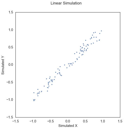
To start, let’s simulate some linear data:
[2]:
x, y = sims.linear_sim(num_samp=100, num_dim=1, noise=0.1)

fig = plt.figure(figsize=(8,8))
fig.suptitle("Linear Simulation", fontsize=17)
ax = sns.scatterplot(x=x[:,0], y=y[:,0])
ax.set_xlabel('Simulated X', fontsize=15)
ax.set_ylabel('Simulated Y', fontsize=15)
plt.axis('equal')
plt.xticks(fontsize=15)
plt.yticks(fontsize=15)
plt.show()
The test statistic and p-value can be called by creating the KendallSpearman object and simply calling the corresponding test statistic and p-value methods. When creating the object, it is necessary to define the which_test parameter so that the correct test is run (Kendall in this case).
[3]:
kendall = KendallSpearman(which_test="kendall")
kendall_statistic, independence_test_metadata = kendall.test_statistic(x, y)
p_value, _ = kendall.p_value(x, y)

print("Kendall test statistic:", kendall_statistic)
print("P Value:", p_value)
Kendall test statistic: 0.8905050505050507
P Value: 2.2897821932369628e-39
Note that Kendall only operates on univariate data.
Spearman’s \(\rho\)
In this tutorial, we explore
The theory behind the Spearman test statistic and p-value
The features of the implementation
Theory
Spearman and Kendall are closely related because they both operate on univariate ranked data. The following description is adapted from [1]:
Spearman can be thought of as closely related to Pearson’s product-moment correlation [5]. Suppose that \(\mathrm{rg}_{x_i}\) and \(\mathrm{rg}_{y_i}\) are the respective ranks of \(n\) raw scores \(x_i\) and \(y_i\), \(\rho\) denotes the Pearson’s coefficient but applied to rank variables, \(\hat{\mathrm{cov}} (\mathrm{rg}_{\mathbf{x}}, \mathrm{rg}_{\mathbf{y}})\) denotes the covariance of the rank variables, and \(\hat{\sigma}_{\mathrm{rg}_{\mathbf{x}}}\) and \(\hat{\sigma}_{\mathrm{rg}_{\mathbf{y}}}\) denote the standard deviations of the rank variables. The statistic is
This implementation wraps scipy.stats.spearmanr [4] to conform to the mgcpy API.
Using Spearman’s \(\rho\)
The test statistic and p-value can be called by creating the KendallSpearman object and simply calling the corresponding test statistic and p-value methods. When creating the object, it is necessary to define the which_test parameter so that the correct test is run (Spearman in this case). Using the same linear relationship as before:
[4]:
spearman = KendallSpearman(which_test="spearman")
spearman_statistic, independence_test_metadata = spearman.test_statistic(x, y)
p_value, _ = spearman.p_value(x, y)

print("Kendall test statistic:", spearman_statistic)
print("P Value:", p_value)
Kendall test statistic: 0.982214221422142
P Value: 5.3309467589776e-73
Note that Spearman only operates on univariate data.