MGC-X and DCorr-X: Independence Testing for Time Series
In this tutorial, we explore
The theory behind the Cross Distance Correlation (DCorr-X) and Cross Multiscale Graph Correlation (MGC-X) tests
The unique methodological features such as optimal scale and optimal lag
The features of the implementation
Theory
Notation
Let \(\mathbb{N}\) be the non-negative integers \(\{0, 1, 2, ...\}\), and \(\mathbb{R}\) be the real line \((-\infty, \infty)\). Let \(F_X\), \(F_Y\), and \(F_{X,Y}\) represent the marginal and joint distributions of random variables \(X\) and \(Y\), whose realizations exist in \(\mathcal{X}\) and \(\mathcal{Y}\), respectively. Similarly, Let \(F_{X_t}\), \(F_{Y_s}\), and \(F_{(X_t,Y_s)}\) represent the marginal and joint distributions of the time-indexed random variables \(X_t\) and \(Y_s\) at timesteps \(t\) and \(s\). For this work, assume \(\mathcal{X} = \mathbb{R}^p\) and \(\mathcal{Y} = \mathbb{R}^q\) for \(p, q > 0\). Finally, let \(\{(X_t,Y_t)\}_{t=-\infty}^{\infty}\) represent the full, jointly-sampled time series, structured as a countably long list of observations \((X_t, Y_t)\).
Problem Statement
The test addresses the problem of independence testing for time series. To formalize the problem, consider a strictly stationary time series \(\{(X_t,Y_t)\}_{t=-\infty}^{\infty}\), with the observed sample \(\{(X_1,Y_1),...,(X_n, Y_n)\}\). Choose some \(M \in \mathbb{N}\), the maximum_lag hyperparameter. We test the independence of two series via the following hypothesis.
The null hypothesis implies that for any \((M+1)\)-length stretch in the time series, \(X_t\) is pairwise independent of present and past values \(Y_{t-j}\) spaced \(j\) timesteps away (including \(j=0\)). A corresponding test for whether \(Y_t\) is dependent on past values of \(X_t\) is available by swapping the labels of each time series. Finally, the hyperparameter \(M\) governs the maximum number of timesteps in the past for which we check the influence of \(Y_{t-j}\) on \(X_t\). This \(M\) can be chosen for computation considerations, as well as for specific subject matter purposes, e.g. a signal from one region of the brain might only influence be able to influence another within 20 time steps implies \(M = 20\).
The Test Statistic
Define the cross-distance correlation at lag \(j\) as
Where \(\text{DCorr}(\cdot, \cdot)\) is the distance correlation function. Assuming strict stationarity of \(\{(X_t,Y_t)\}\) is important in even defining \(\text{DCorr}(j)\), as the parameter depends only on the spacing \(j\), and not the timestep \(t\) of \(X_t\) and \(Y_{t-j}\). Similarly, let \(\text{DCorr}n(j)\) be its estimator, with \(\text{MGC}_n(j)\) being the \(\text{MGC}\) test statistic evaluated for \(\{X_t\}\) and \(\{Y_{t-j}\}\). The \(\text{DCorr-X}^M\) test statistic is
Similarly, the \(\text{MGC-X}\) test statistic is
While \(\text{MGC-X}\) is more computationally intensive than \(\text{DCorr-X}\), \(\text{MGC-X}\) employs multiscale analysis to achieve better finite-sample power in high-dimensional, nonlinear, and structured data settings [1].
The P-Value
Let \(T_n\) represent either of the test statistics above. To compute the p-value, one need to estimate the null distribution of \(T_n\), namely its distribution under indepdendence pair of data. A typical permutation test would permute the indices \(\{1,2,3,...,n\}\), reorder the series \(\{Y_t\}\) according to this permutation, and \(T_n\) would be computed on \(\{X_t\}\) and the reordered \(\{Y_t\}\). This procedure would be repeated \(K\) times, generating \(K\) samples of the test statistic under the null. This permutation test requires exchangeability of the sequence \(\{Y_t\}\), which would be true in the i.i.d. case, but is generally violated in the time series case. Instead, a block permutation captures the dependence between elements of the series, as described in \cite{politis2003}. Letting \(\lceil \cdot \rceil\) be the ceiling function, this procedure partitions the list of indices into size \(b\) “blocks”, and permutes the \(\lceil \frac{n}{b} \rceil\) blocks in order to generate samples of the test statistic under the null. Specifically,
Choose a random permutation of the indices \(\{0, 1, 2, ..., \lceil \frac{n}{b} \rceil\}\).
From index \(i\) in the permutation, produce block \(B_{i} = (Y_{bi+1},Y_{bi+2},...,Y_{bi + b})\), which is a section of the series \(\{Y_t\}\).
Let the series \(\{Y_{\pi(1)}, ..., Y_{\pi(n)}\} = (B_1, B_2, ..., B_{\frac{n}{b}})\), where \(\pi\) maps indices \(\{1,2,...,n\}\) to the new, block permuted indices.
Compute \(T^{(r)}_n\) on the series \(\{(X_t, Y_{\pi(t)})\}_{t=1}^n\) for replicate \(r\).
Repeat this procedure \(K\) times (typically \(K = 100\) or \(1000\)), and let \(T^{(0)}_n = T_n\), with:
where \(\mathbb{I}\{\cdot\}\) is the indicator function.
Using DCorr-X and MGC-X
[1]:
%matplotlib inline
import numpy as np
import matplotlib.pyplot as plt
import random
from scipy.stats import pearsonr

from mgcpy.independence_tests.dcorrx import DCorrX
from mgcpy.independence_tests.mgcx import MGCX
Simulate time series
Let \(\epsilon_t\) and \(\eta_t\) be i.i.d. standard normally distributed.
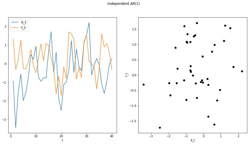
Independent AR(1):
[2]:
def indep_ar1(n, phi = 0.5, sigma2 = 1.0):
    # X_t and Y_t are univarite AR(1) with phi = 0.5 for both series.
    # Noise follows N(0, sigma2).

    # Innovations.
    epsilons = np.random.normal(0.0, sigma2, n)
    etas = np.random.normal(0.0, sigma2, n)

    X = np.zeros(n)
    Y = np.zeros(n)
    X[0] = epsilons[0]
    Y[0] = etas[0]

    # AR(1) process.
    for t in range(1,n):
        X[t] = phi*X[t-1] + epsilons[t]
        Y[t] = phi*Y[t-1] + etas[t]

    return X, Y
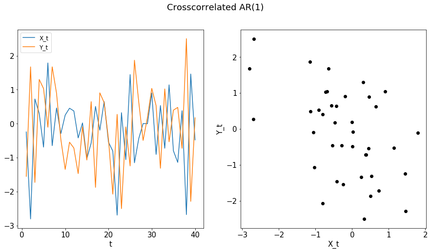
Crosscorrelated AR(1):
[3]:
def cross_corr_ar1(n, phi = 0.5, sigma2 = 1.0):
    # X_t and Y_t are together a bivarite AR(1) with Phi = [0 0.5; 0.5 0].
    # Innovations follow N(0, sigma2).

    # Innovations.
    epsilons = np.random.normal(0.0, sigma2, n)
    etas = np.random.normal(0.0, sigma2, n)

    X = np.zeros(n)
    Y = np.zeros(n)
    X[0] = epsilons[0]
    Y[0] = etas[0]

    for t in range(1,n):
        X[t] = phi*Y[t-1] + epsilons[t]
        Y[t] = phi*X[t-1] + etas[t]

    return X, Y
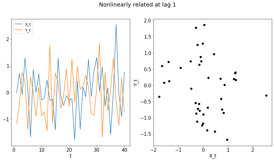
Nonlinearly related at lag 1:
[4]:
def nonlinear_lag1(n, phi = 1, sigma2 = 1):
    # X_t and Y_t are together a bivarite nonlinear process.
    # Innovations follow N(0, sigma2).

    # Innovations.
    epsilons = np.random.normal(0.0, sigma2, n)
    etas = np.random.normal(0.0, sigma2, n)

    X = np.zeros(n)
    Y = np.zeros(n)
    Y[0] = etas[0]

    for t in range(1,n):
        X[t] = phi*epsilons[t]*Y[t-1]
        Y[t] = etas[t]

    return X, Y
Plot time series
[5]:
def plot_ts(X, Y, title, xlab = "X_t", ylab = "Y_t"):
    n = X.shape[0]
    t = range(1, n + 1)

    fig, (ax1, ax2) = plt.subplots(1, 2, figsize=(15,7.5))
    fig.suptitle(title)
    plt.rcParams.update({'font.size': 15})

    ax1.plot(t, X)
    ax1.plot(t, Y)
    ax1.legend(['X_t', 'Y_t'], loc = 'upper left', prop={'size': 12})
    ax1.set_xlabel("t")

    ax2.scatter(X,Y, color="black")
    ax2.set_ylabel(ylab)
    ax2.set_xlabel(xlab)
Explore with DCorr-X and MGC-X.
[6]:
def compute_dcorrx(X, Y, max_lag):
    dcorrx = DCorrX(max_lag = max_lag, which_test = 'unbiased')
    dcorrx_statistic, metadata = dcorrx.test_statistic(X, Y)
    p_value, _ = dcorrx.p_value(X, Y)
    optimal_lag = metadata['optimal_lag']

    print("DCorrX test statistic:", dcorrx_statistic)
    print("P Value:", p_value)
    print("Optimal Lag:", optimal_lag)

def compute_mgcx(X, Y, max_lag):
    mgcx = MGCX(max_lag = max_lag)
    mgcx_statistic, metadata = mgcx.test_statistic(X, Y)
    p_value, _ = mgcx.p_value(X, Y)
    optimal_lag = metadata['optimal_lag']
    optimal_scale = metadata['optimal_scale']

    print("MGCX test statistic:", mgcx_statistic)
    print("P Value:", p_value)
    print("Optimal Lag:", optimal_lag)
    print("Optimal Scale:", optimal_scale)
[7]:
n = 40
max_lag = 0

X, Y = indep_ar1(n)
plot_ts(X, Y, "Independent AR(1)")
compute_dcorrx(X, Y, max_lag)
compute_mgcx(X, Y, max_lag)
DCorrX test statistic: 0.0
P Value: 0.418
Optimal Lag: 0
MGCX test statistic: 0.0
P Value: 0.424
Optimal Lag: 0
Optimal Scale: [40, 40]
In the crosscorrelated time series, the linear dependence will not be apparent at lag 0, but will be at lag 1.
[8]:
n = 40
max_lag = 0

X, Y = cross_corr_ar1(n)
plot_ts(X, Y, "Crosscorrelated AR(1)")
compute_dcorrx(X, Y, max_lag)
compute_mgcx(X, Y, max_lag)
DCorrX test statistic: 0.14380139143970183
P Value: 0.028
Optimal Lag: 0
MGCX test statistic: 0.14550875825340037
P Value: 0.069
Optimal Lag: 0
Optimal Scale: [40, 40]
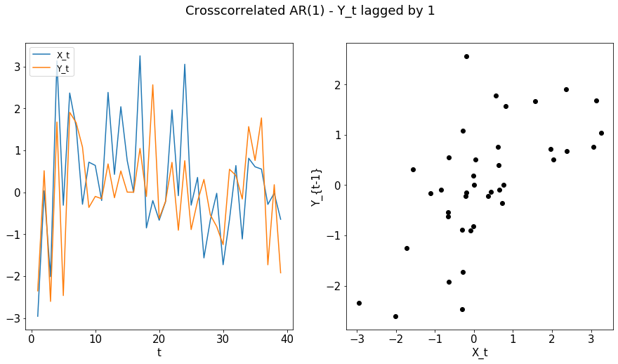
[9]:
max_lag = 1

X, Y = cross_corr_ar1(n)
plot_ts(X[1:n], Y[0:(n-1)], "Crosscorrelated AR(1) - Y_t lagged by 1", ylab = "Y_{t-1}")
compute_dcorrx(X, Y, max_lag)
compute_mgcx(X, Y, max_lag)
DCorrX test statistic: 0.35649077356316006
P Value: 0.003
Optimal Lag: 1
MGCX test statistic: 0.35511264701472667
P Value: 0.012
Optimal Lag: 1
Optimal Scale: [39, 39]
The final example is a nonlinearly related series, for which the Pearson’s correlation may be insufficient.
[10]:
X, Y = nonlinear_lag1(n)

print("Pearson's Correlation at lag 0: " + str(pearsonr(X,Y)[0]))
print("Pearson's Correlation at lag 1: " + str(pearsonr(X[1:n],Y[0:(n-1)])[0]))
Pearson's Correlation at lag 0: -0.16740183702829184
Pearson's Correlation at lag 1: 0.2840269513248397
[11]:
plot_ts(X, Y, "Nonlinearly related at lag 1")
compute_dcorrx(X, Y, max_lag)
compute_mgcx(X, Y, max_lag)
DCorrX test statistic: 0.07967130243446058
P Value: 0.159
Optimal Lag: 1
MGCX test statistic: 0.35820807204909766
P Value: 0.008
Optimal Lag: 0
Optimal Scale: [35, 13]
Understanding the Optimal Lag
The optimal lag allows the user to understand better the temporal nature of the relationship between \(X_t\) and \(Y_t\). The polt below shows the empirical distribution of the optimal lag estimate for \(\text{MGC-X}\) as \(n\) increases.
[12]:
# Plot the distribution of optimal lag estimates.
def opt_lag_dist(optimal_lags_dcorrx, optimal_lags_mgcx, n, M = 10):
    fig, (ax1, ax2) = plt.subplots(1, 2, figsize=(15,7.5), sharey = True)
    plt.rcParams.update({'font.size': 15})

    ax1.set_xlabel('Lag j')
    ax1.set_title("DCorr-X, n = %d" % n)
    ax2.set_xlabel('Lag j')
    ax2.set_title("MGC-X, n = %d" % n)
    ax1.set_ylabel("Freq. of Optimal Lag Estimates")

    # Optimal lag predictions.
    weights = np.ones_like(optimal_lags_dcorrx)/float(len(optimal_lags_dcorrx))
    ax1.hist(optimal_lags_dcorrx,
             bins = np.arange(M)-0.5,
             weights = weights,
             align = 'mid',
             edgecolor ='black',
             color = 'blue')
    weights = np.ones_like(optimal_lags_mgcx)/float(len(optimal_lags_mgcx))
    ax2.hist(optimal_lags_mgcx,
             bins = np.arange(M)-0.5,
             weights = weights,
             align = 'mid',
             edgecolor ='black',
             color = 'red')

    plt.show()
We simulate a nonlinear process that has clear dependence at lag 3.
[13]:
def nonlinear_lag3(n, phi = 1, sigma2 = 1):
    # X_t and Y_t are together a bivarite nonlinear process.
    # Innovations follow N(0, sigma2).

    # Innovations.
    epsilons = np.random.normal(0.0, sigma2, n)
    etas = np.random.normal(0.0, sigma2, n)

    X = np.zeros(n)
    Y = np.zeros(n)
    for t in range(3):
        Y[t] = etas[t]

    for t in range(3,n):
        X[t] = phi*epsilons[t]*Y[t-3]
        Y[t] = etas[t]

    return X, Y
[14]:
M = 10
num_sims = 100

dcorrx = DCorrX(max_lag = M)
mgcx = MGCX(max_lag = M)
optimal_lags_dcorrx = np.zeros(num_sims)
optimal_lags_mgcx = np.zeros(num_sims)

# Run experiments.
for n in [15, 30, 60]:
    for t in range(num_sims):
        X, Y = nonlinear_lag3(n)
        test_statistic, metadata = dcorrx.test_statistic(X, Y)
        optimal_lags_dcorrx[t] = metadata['optimal_lag']
        test_statistic, metadata = mgcx.test_statistic(X, Y)
        optimal_lags_mgcx[t] = metadata['optimal_lag']
    opt_lag_dist(optimal_lags_dcorrx, optimal_lags_mgcx, n)
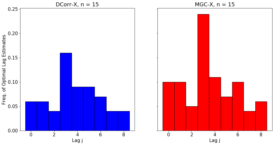
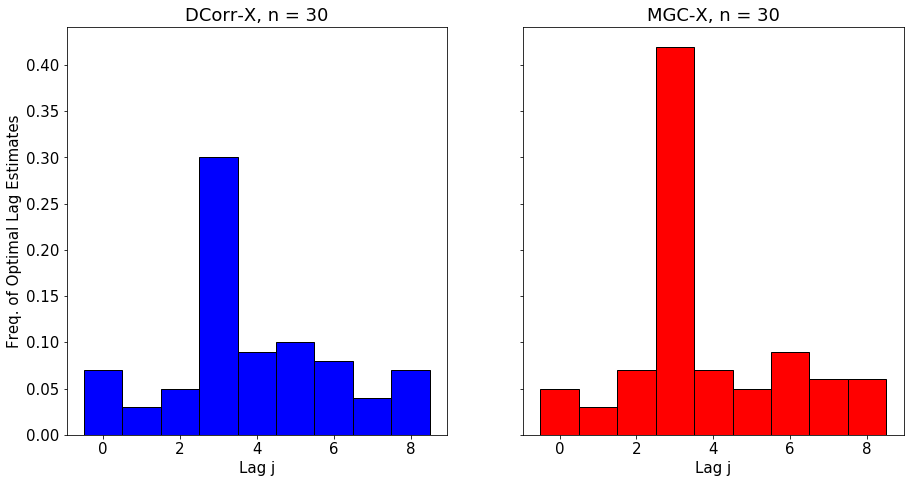
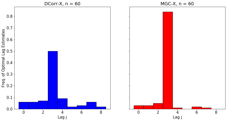
DCorrX and MGCX both close in on the correct lag as n increases, with MGCX having higher accuracy due to advantages in nonlinear settings.