Simulations

In this tutorial, we explore

• The mathematical representations of the simulations

• Plots showing each simulation

Mathematical Equations

Simulations for the power curves were generated using the following equations:

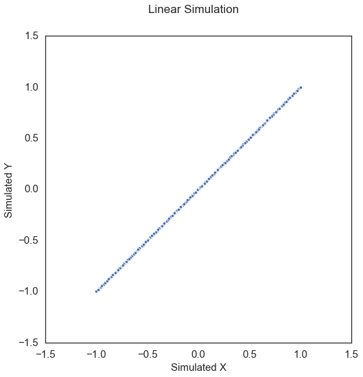
• Linear\(\left( X, Y \right) \in \mathbb{R}^p \times \mathbb{R}\):

\[X \sim {\mathcal{U} \left( -1, 1 \right)}^p,\]

\[Y = w ^T X + \kappa \epsilon.\]

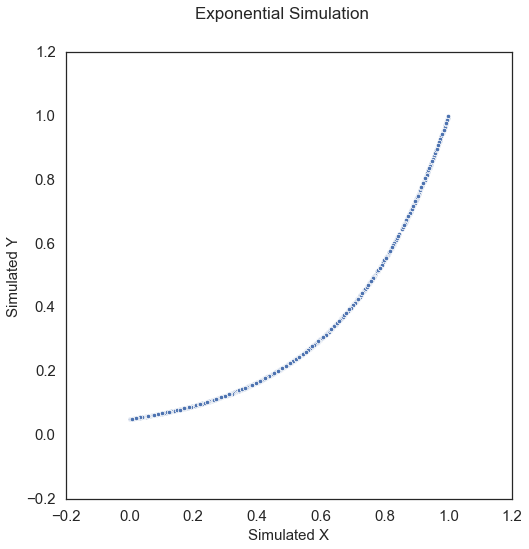
• Exponential\(\left( X, Y \right) \in \mathbb{R}^p \times \mathbb{R}\):

\[X \sim {\mathcal{U} \left( 0, 3 \right)}^p,\]

\[Y = \exp \left( w ^T X \right) + 10 \kappa \epsilon.\]

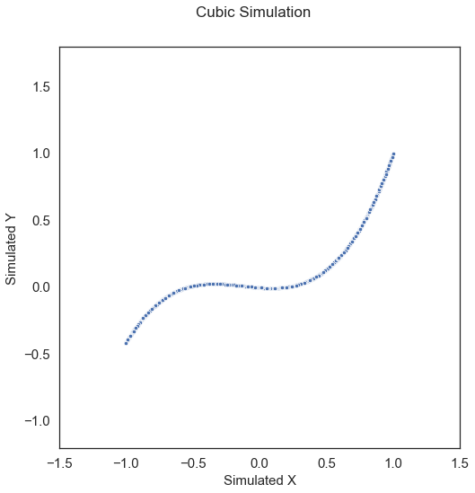
• Cubic\(\left( X, Y \right) \in \mathbb{R}^p \times \mathbb{R}\):

\[X \sim {\mathcal{U} \left( -1, 1 \right)}^p,\]

\[Y = 128 {\left( w ^T X - \frac{1}{3} \right)}^3 + 48 {\left( w ^T X - \frac{1}{3} \right)}^2 - 12 \left( w ^T X - \frac{1}{3} \right) + 80 \kappa \epsilon.\]

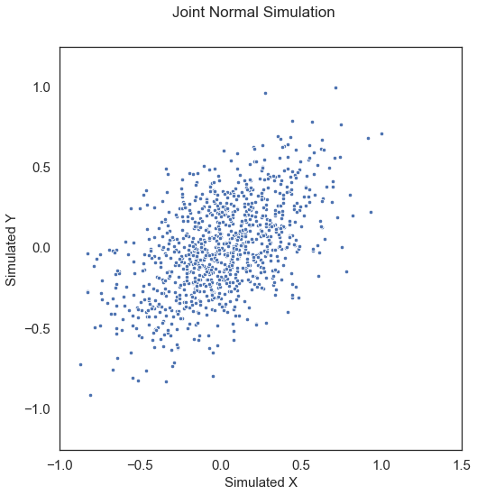
• Joint Normal\(\left ( X, Y \right) \in \mathbb{R}^p \times \mathbb{R}^p\): Let \(\rho = 1/2 p\), \(I_p\) be the identity matrix of size \(p \times p\), \(J_p\) be the matrix of ones of size \(p \times p\), and \(\Sigma = \begin{bmatrix} I_p & \rho J_p \\ \rho J_p & \left(1 + 0.5 \kappa \right) I_p\\ \end{bmatrix}\). Then,

\[\left( X, Y \right) \sim \mathcal{N} \left( 0, \Sigma \right).\]

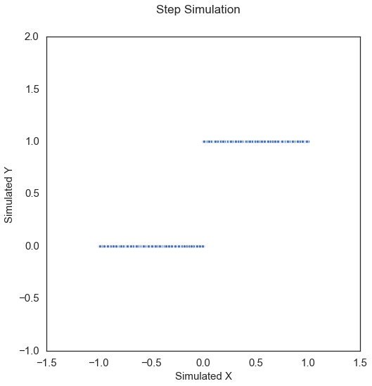
• Step Function\(\left( X, Y \right) \in \mathbb{R}^p \times \mathbb{R}\):

\[X \sim {\mathcal{U} \left( -1, 1 \right)}^p,\]

\[Y = \mathcal{I} \left( w ^T X > 0 \right) + \epsilon,\]

where \(\mathcal{I}\) is the indicator function, that is \(\mathcal{I} \left( z \right)\) is unity whenever \(z\) is true, and \(0\) otherwise.

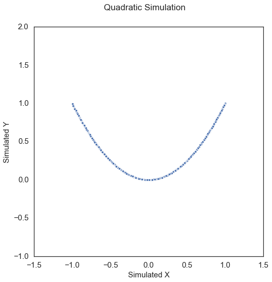
• Quadratic\(\left( X, Y \right) \in \mathbb{R}^p \times \mathbb{R}\):

\[X \sim {\mathcal{U} \left( -1, 1 \right)}^p,\]

\[Y = {\left( w ^T X \right)}^2 + 0.5 \kappa \epsilon.\]

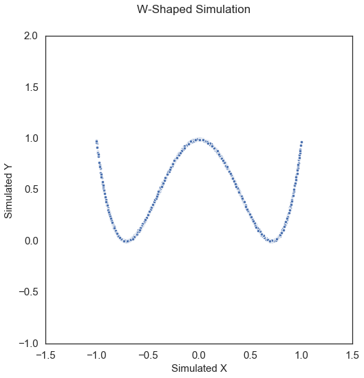
• W-Shape\(\left( X, Y \right) \in \mathbb{R}^p \times \mathbb{R}\): For \(U \sim {\mathcal{U} \left( -1, 1 \right)}^p\),

\[X \sim {\mathcal{U} \left( -1, 1 \right)}^p,\]

\[Y = 4 \left[ {\left( {\left( w ^T X \right)}^2 - \frac{1}{2} \right)}^2 + \frac{w ^T U}{500} \right] + 0.5 \kappa \epsilon.\]

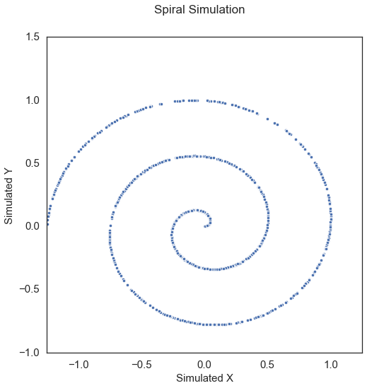
• Spiral\(\left( X, Y \right) \in \mathbb{R}^p \times \mathbb{R}\): For \(U \sim \mathcal{U} \left( 0, 5 \right)\), \(\epsilon \sim \mathcal{N} \left( 0, 1 \right)\),

\[X_{\left| d \right|} = U \sin \left(\pi U \right) \cos^d \left(\pi U \right)\ \mathrm{for}\ d = 1, ..., p - 1,\]

\[X_{\left| p \right|} = U \cos^p \left(\pi U \right),\]

\[Y = U \sin \left( \pi U \right) + 0.4 p \epsilon.\]

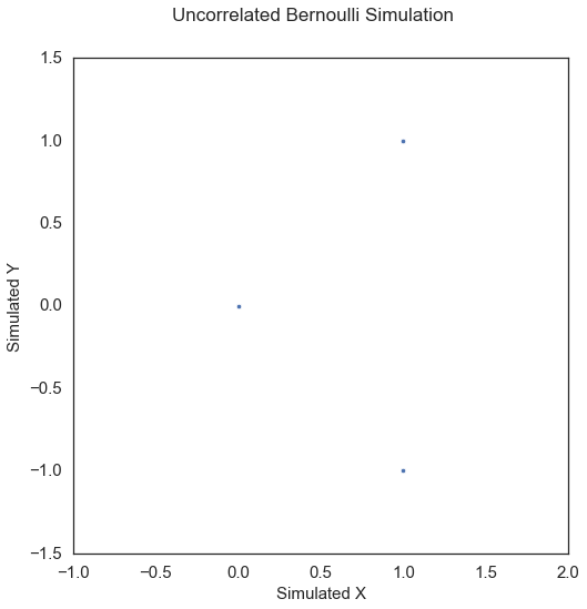
• Uncorrelated Bernoulli\(\left( X, Y \right) \in \mathbb{R}^p \times \mathbb{R}\): For \(U \sim \mathcal{B} \left( 0.5 \right)\), \(\epsilon_1 \sim \mathcal{N} \left( 0, I_p \right)\), \(\epsilon_2 \sim \mathcal{N} \left( 0, 1 \right)\),

\[X \sim {\mathcal{B} \left( 0.5 \right)}^p + 0.5 \epsilon_1,\]

\[Y = \left( 2 U - 1 \right) w ^T X + 0.5 \epsilon_2.\]

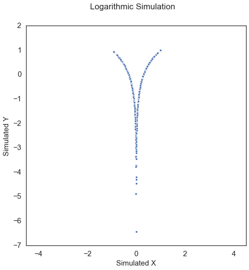
• Logarithmic\(\left( X, Y \right) \in \mathbb{R}^p \times \mathbb{R}^p\): For \(\epsilon \sim \mathcal{N} \left( 0, I_p \right)\),

\[X \sim \mathcal{N} \left( 0, I_p \right),\]

\[Y_{\left| d \right|} = 2 \log_2 \left( \left| X_{\left| d \right|} \right| \right) + 3 \kappa \epsilon_{\left| d \right|}\ \mathrm{for}\ d = 1, ..., p.\]

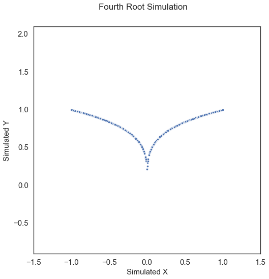
• Fourth Root\(\left( X, Y \right) \in \mathbb{R}^p \times \mathbb{R}\):

\[X \sim {\mathcal{U} \left( -1, 1 \right)}^p,\]

\[Y = {\left| w ^T X \right|}^{1/4} + \frac{\kappa}{4} \epsilon.\]

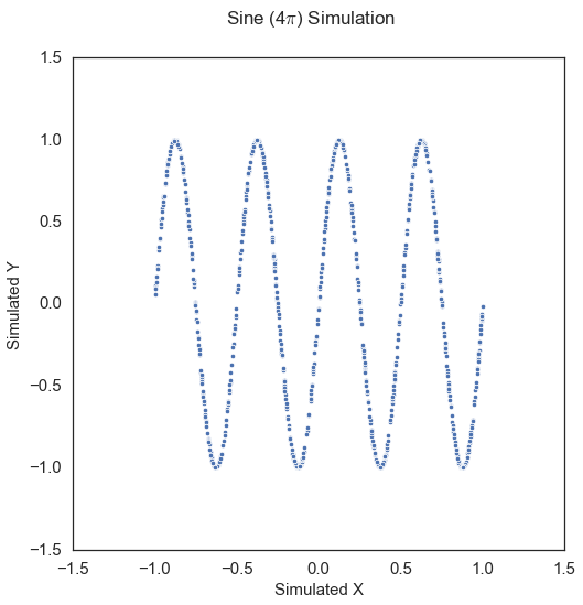
• Sine Period 4\(\pi\) \(\left( X, Y \right) \in \mathbb{R}^p \times \mathbb{R}^p\): For \(U \sim \mathcal{U} \left( -1, 1 \right)\), \(V \sim {\mathcal{N} \left( 0, 1 \right)}^p\), \(\theta = 4 \pi\),

\[X_{\left| d \right|} = U + 0.02 p V_{\left| d \right|}\ \mathrm{for}\ d = 1, ..., p,\]

\[Y=\sin(\theta X)+\kappa \epsilon.\]

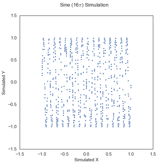
• Sine Period 16\(\pi\) \(\left( X, Y \right) \in \mathbb{R}^p \times \mathbb{R}^p\): Same as above except \(\theta = 16 \pi\) and the noise on \(Y\) is changed to \(0.5 \kappa \epsilon\).

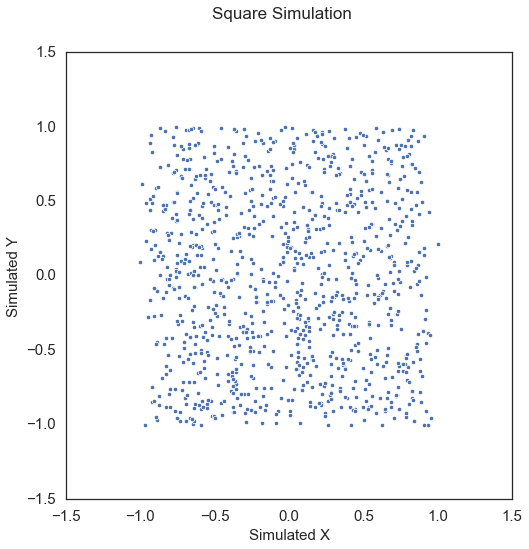
• Square\(\left( X, Y \right) \in \mathbb{R}^p \times \mathbb{R}^p\): For \(U \sim \mathcal{U} \left( -1, 1 \right)\), \(V \sim \mathcal{U} \left( -1, 1 \right)\), \(\epsilon \sim {\mathcal{N} \left( 0, 1 \right)}^p\), \(\theta = -\frac{\pi}{8}\),

\[X_{\left| d \right|} = U \cos \left( \theta \right) + V \sin \left( \theta \right) + 0.05 p \epsilon_{\left| d \right|},\]

\[Y_{\left| d \right|} = -U \sin \left( \theta \right) + V \cos \left( \theta \right).\]

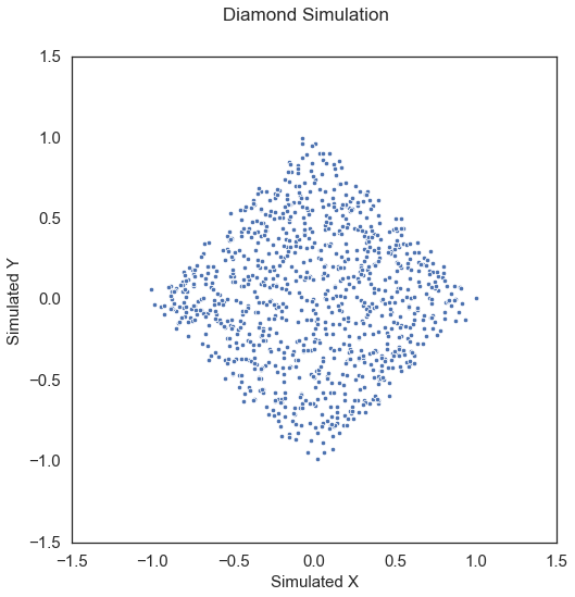
• Diamond\(\left( X, Y \right) \in \mathbb{R}^p \times \mathbb{R}^p\): Same as above except \(\theta = \pi/4\).

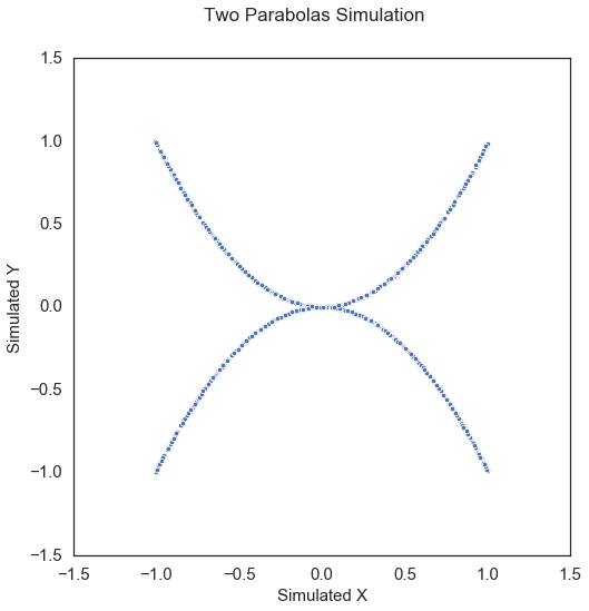
• Two Parabolas\(\left( X, Y \right) \in \mathbb{R}^p \times \mathbb{R}\): For \(\epsilon \sim \mathcal{U} \left( 0, 1 \right)\), \(U \sim \mathcal{B} \left( 0.5 \right)\),

\[X \sim {\mathcal{U} \left( -1, 1 \right)}^p,\]

\[Y = \left( {\left( w ^T X \right)}^2 + 2 \kappa \epsilon \right) \cdot \left(U - \frac{1}{2} \right).\]

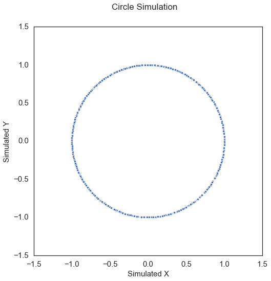
• Circle\(\left( X, Y \right) \in \mathbb{R}^p \times \mathbb{R}\): For \(U \sim {\mathcal{U} \left( -1, 1 \right)}^p\), \(\epsilon \sim \mathcal{N} \left( 0, I_p \right)\), \(r = 1\),

\[X_{\left| d \right|} = r \left( \sin \left( \pi U_{\left| d + 1 \right|} \right) \prod \limits_{j = 1}^d \cos \left( \pi U_{\left| j \right|} \right) + 0.4 \epsilon_{\left| d \right|} \right)\ \mathrm{for}\ d = 1, ..., p-1,\]

\[X_{\left| d \right|} = r \left( \prod \limits_{j = 1}^p \cos \left(\pi U_{\left| j \right|} \right) + 0.4 \epsilon_{\left| p \right|} \right),\]

\[Y_{\left| d \right|} = \sin \left(\pi U_{\left| 1 \right|} \right).\]

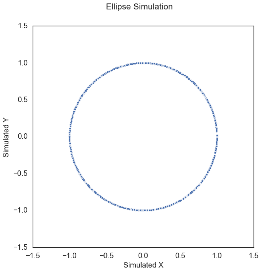
• Ellipse\(\left( X, Y \right) \in \mathbb{R}^p \times \mathbb{R}^p\): Same as above except \(r = 5\).

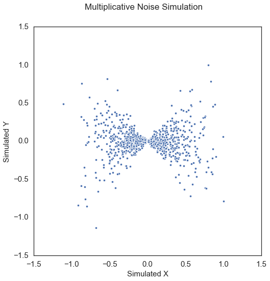
• Multiplicative Noise\(\left( x, y \right) \in \mathbb{R}^p \times \mathbb{R}^p\): \(u \sim \mathcal{N} \left( 0, I_p \right)\),

\[x \sim \mathcal{N} \left( 0, I_p \right),\]

\[y_{\left| d \right|} = u_{\left| d \right|} x_{\left| d \right|}\ \mathrm{for}\ d = 1, ..., p.\]

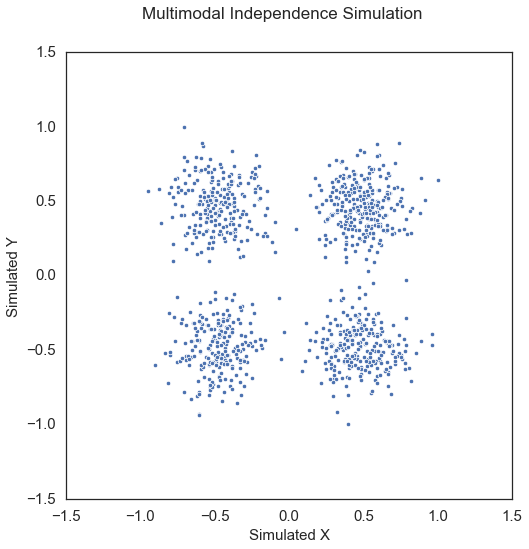
• Multimodal Independence\(\left( X, Y \right) \in \mathbb{R}^p \times \mathbb{R}\): For \(U \sim \mathcal{N} \left( 0, I_p \right)\), \(V \sim \mathcal{N} \left( 0, I_p \right)\), \(U' \sim {\mathcal{B} \left( 0.5 \right)}^p\), \(V' \sim {\mathcal{B} \left( 0.5 \right)}^p\),

\[X = U/3 + 2U' - 1,\]

\[Y = V/3 + 2V' - 1.\]

Plots

Let’s import some useful packages and create a function that plots our simulated 1D data, to ensure consistency in these examples, we set the seed:

%matplotlib inline
import numpy as np
import matplotlib.pyplot as plt; plt.style.use('classic')
import seaborn as sns; sns.set(style="white")

from mgcpy.benchmarks.simulations import *

np.random.seed(12345678)

def plot_sims(sim_name, sim_func):
    """
    Plots all of the simulations
    """
    if sim_name == 'Sine (16$\pi$)':
        x, y = sim_func(num_samp=1000, num_dim=1, noise=0, period=16*np.pi)
    elif sim_name == 'Ellipse':
        x, y = sim_func(num_samp=1000, num_dim=1, noise=0, radius=5)
    elif sim_name == 'Diamond':
        x, y = sim_func(num_samp=1000, num_dim=1, noise=0, period=-np.pi/4)
    elif sim_name == 'Multiplicative Noise' or sim_name == 'Multimodal Independence':
        x, y = sim_func(num_samp=1000, num_dim=1)
    else:
        x, y = sim_func(num_samp=1000, num_dim=1, noise=0)

    # Normalize
    x = x / np.max(x)
    y = y / np.max(y)

    fig = plt.figure(figsize=(8,8))
    fig.suptitle(sim_name + " Simulation", fontsize=17)
    ax = sns.scatterplot(x=x[:,0], y=y[:,0])
    ax.set_xlabel('Simulated X', fontsize=15)
    ax.set_ylabel('Simulated Y', fontsize=15)
    plt.axis('equal')
    plt.xticks(fontsize=15)
    plt.yticks(fontsize=15)
    plt.show()

Simultions are randomly generated with an \(x\) which is \((n \times d)\) and \(y\) which is \((n \times 1)\) that have 2 required parameters: num_samp or the number of samples, and num_dim or the number of dimensions. Optional parameters can be set based on the documentation. Visualizations of are shown below with and without the noise. Here are all the simulations:

sim_func = [linear_sim, exp_sim, cub_sim, joint_sim, step_sim, quad_sim, w_sim, spiral_sim, ubern_sim, log_sim,
            root_sim, sin_sim, sin_sim, square_sim, two_parab_sim, circle_sim, circle_sim, square_sim,
            multi_noise_sim, multi_indep_sim]
sim_name = ['Linear', 'Exponential', 'Cubic', 'Joint Normal', 'Step', 'Quadratic', 'W-Shaped', 'Spiral',
            'Uncorrelated Bernoulli', 'Logarithmic', 'Fourth Root', 'Sine (4$\pi$)', 'Sine (16$\pi$)', 'Square',
            'Two Parabolas', 'Circle', 'Ellipse', 'Diamond', 'Multiplicative Noise', 'Multimodal Independence']

for i in range(len(sim_func)):
    plot_sims(sim_name[i], sim_func[i])